Interactive fish phylogeny

The Betancur-R bony fish phylogeny, visualized in anvi’o, with metadata scraped from FishBase using rvest.

9 Jan 2020

Table of Contents

All banner images from The Fishes of Porto Rico (1902) by Everman & Marsh, Bulletin of the United States Fish Commission, v.20, pt.1, for 1900, Washington, DC: Government Printing Office. Retrieved from Wikimedia Commons and licenced under CC-0. Yes, that is how they spelled Puerto Rico in 1902.

My goal in this project is to extend the functionality of the phylogeny of bony fishes by Betancur-R et. al., (2017). I use anvi’o to visualize the tree and metadata scraped from FishBase to create an interactive phylogeny.

If you are only interested in the data, no need to read further. You can grab all the files from the GitHub repo linked above or by clicking here. The repo contains instructions and files needed to visualize the Betancur-R and the FishBase metadata in anvi’o.

Background

As part of an analysis for another project, I needed to create a phylogenetic tree of five fish species. To construct the tree, I also needed an appropriate out group, but given that I knew little about fish, I wasn’t sure which species would be most appropriate. My search for an out-group lead to DeepFin and the amazing paper by Betancur-R et. al.(2017) about the phylogenetic classification of bony fishes.

Anyway, I used the tree from the paper to choose Gerreidae as the out group for the analysis. I then decided to make my own interactive representation of the Betancur-R tree using anvi’o. Anvi’o is an open-source, community-driven analysis and visualization platform for ‘omics data. One of the best aspects of anvi’o is its interactive interface, which is amazing for data exploration—including phylogenetic trees. Another strength of the interface is that you can overlay all types of metadata. I wanted to capitalize on this functionality and gathered as much metadata as I could for each species. For this part I used the R package rvest to scrape species pages on FishBase for metadata.

How I did all of this is the subject of this post.

Workflow overview

Get the Betancur-R tree data.
Modify the data to be compatible with anvi’o.
Scrape FishBase for metadata using rvest in R.
Curate metadata. Some manual manipulation required.
Build anvi’o profile data base.

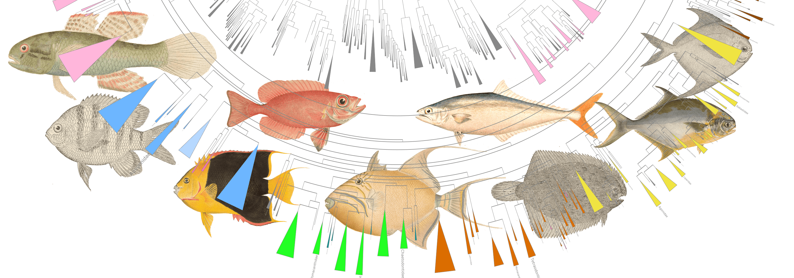
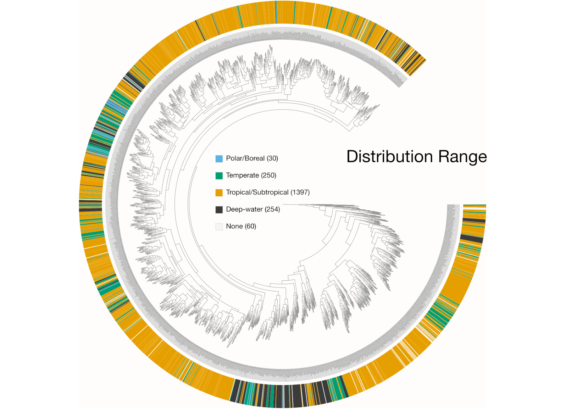
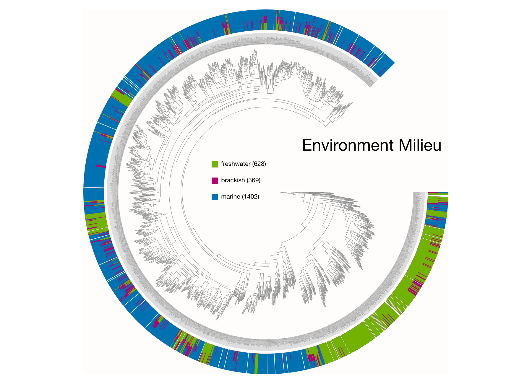
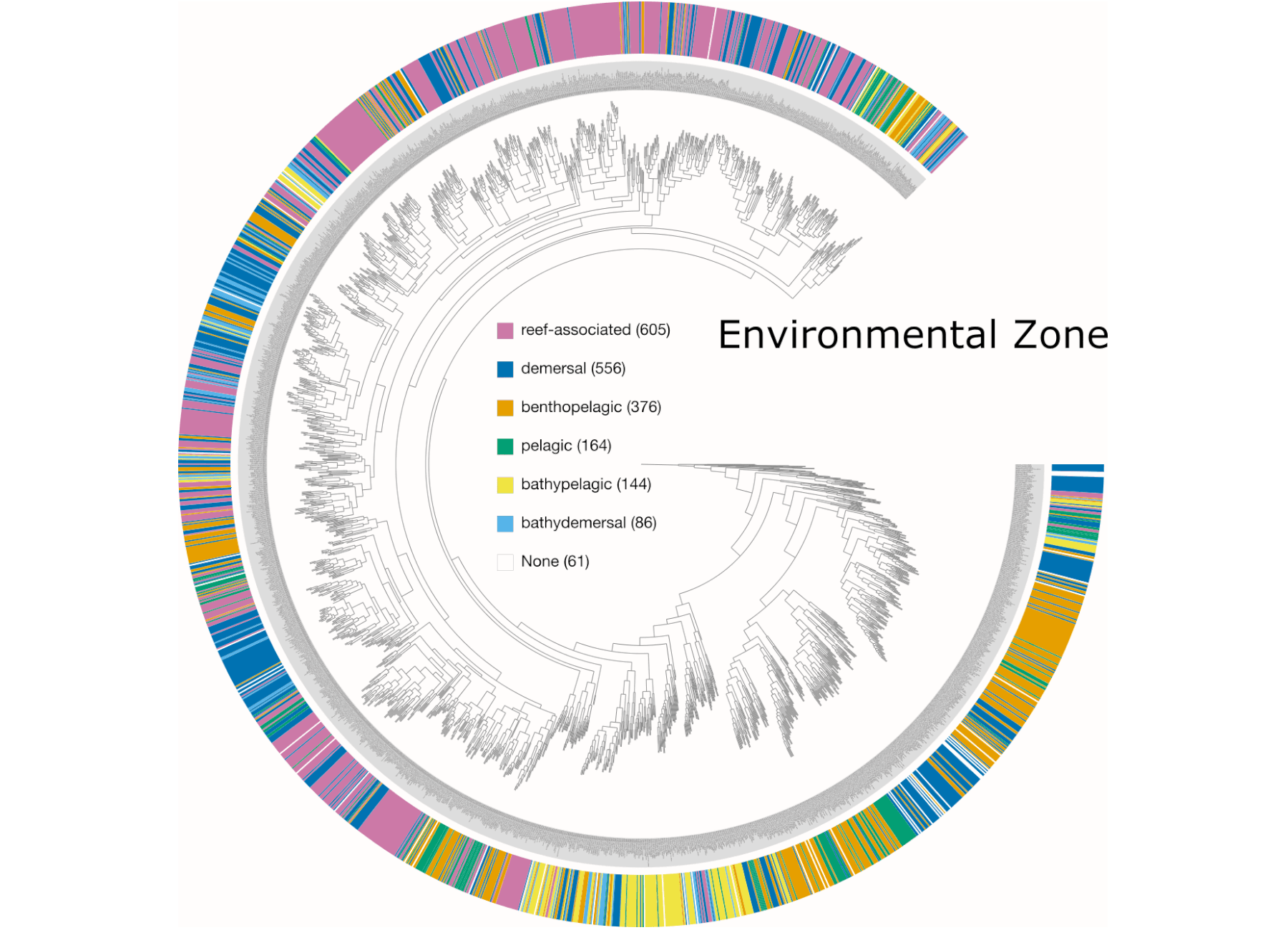
Examples of viualization in anvi’o

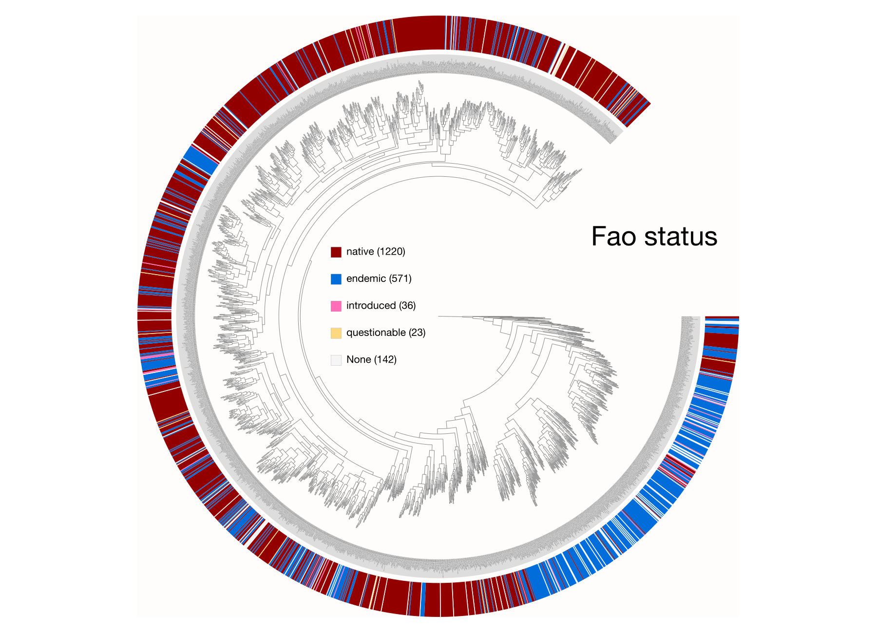
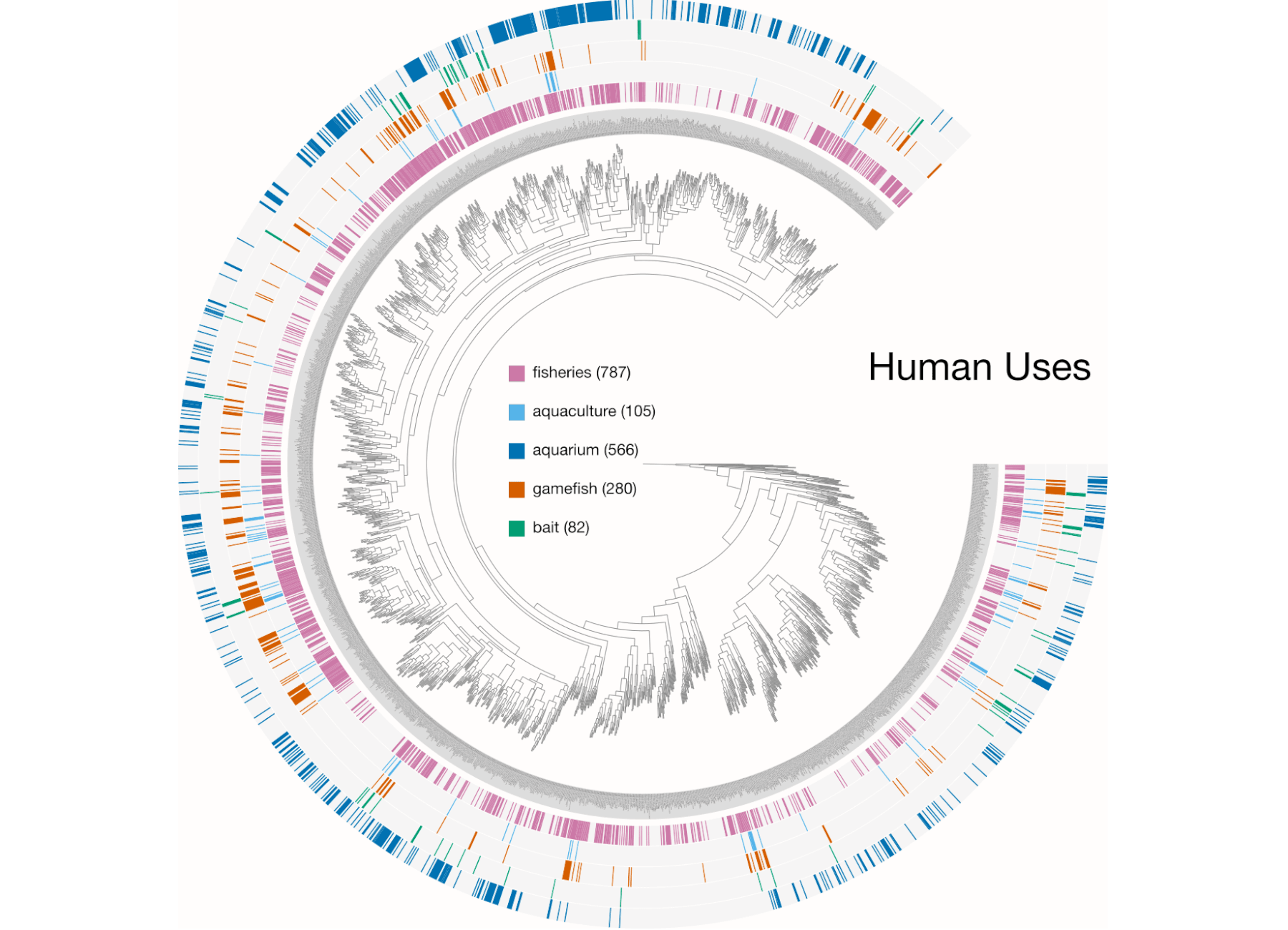
Here are a few examples of the Betancur-R tree, accompanied by various pieces of FishBase metadata, all visualized in anvi’o.

The Betancur-R Fish Phylogeny Data

The Betancur-R bony fish phylogeny from the paper is the 4th version (the original dates back to 2013) and contains 1992 species encompassing 72 orders and 410 families. Wow. The tree has representatives from roughly 80% of recognized bony fish families. The study used molecular and genomic data to base classification on inferred phylogenies. From the abstract the author states:

The first explicit phylogenetic classification of bony fishes was published in 2013, based on a comprehensive molecular phylogeny (www.deepfin.org). We here update the first version of that classification by incorporating the most recent phylogenetic results.

The authors provide many files with the paper but for the purposes of this visualization I used two files from the Supplementary material, specifically Additional file 2 (complete tree in newick format) and Additional file 4 (Table S1. spreadsheet with full classification).

I first modified the tree file slightly—in the original file, the Family name was used as a prefix for each species. I removed the Family names from all leaves. To do this you could of course use the command line, but I prefer using the BBEdit text editor because it allows grep pattern matching and I can see what is being replaced before I do anything. Plus, for some reason I still absolutely terrible at using the command line for find and replace functions. So, there’s that too. The free version of BBEdit has this functionality but if you like the software I recommend purchasing a one-time license. Anyway, this simple regular expression will replace all the Family names in the tree.

[A-Z]\w+ae_

Basically, the command says look for a single capital letter ([A-Z]), followed by any word character (\w) any number of times (+), then the letters ae, and finally an underscore (_). The ae is important because all of the Family names end in ae.

I also removed any subspecies names and any other superfluous information.

Scraping FishBase

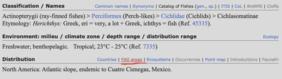
The next step was to collect metadata about each fish to include in the visualization. FishBase is a huge online data base and as of this writing had information on over 34,000 fish species. Here is an example page about Herichthys minckleyi or Minkley’s cichlid, a freshwater fish endemic to Cuatro Cienegas, Mexico. There is a lot of metadata on these pages, but I was specifically interested in the following pieces:

the scientific and common names.
the Environment metadata.
the Size / Weight / Age metadata.
the IUCN Red List Status.
the Threat to humans.
the Human uses.
the Distribution metadata. Note this is retrieved separately.

Given the size of the tree, doing all of this by hand was simply out of the question. So, I had to learn a little about web scraping. I will not go into the details of web scraping here but basically I used HTML parsing, where specific sequences of HTML tags are used to parse information. The great thing about FishBase is that species pages follow the same general format, making it easier to grab the info you want. Ultimately, how you code a web scrape is highly dependent on structure of the page and the info you want. If you are interested in web scraping there are a ton of great resources and courses. Here are a few I relied on heavily.

Web crawling and scraping from a tutorial on Text mining in R for the social sciences and digital humanities by Andreas Niekler, Gregor Wiedemann.
Web Scraping Reference: Cheat Sheet for Web Scraping using R by yifyan.
R Web Scraping Cheat Sheet from Awesome Open Source.
Functions with R and rvest: A Laymen’s Guide by @peterjgensler. This article was key in helping me design the functions described below.

This workflow uses rvest, an R package for scraping web pages. I will keep the explanation here to a minimum since there are many authoritative sources online.

The first thing to do is load the required packages.

library(tidyverse)
library(webdriver)
library(magrittr)
library(dplyr)
library(rvest)
library(xml2)
library(selectr)
library(tibble)
library(purrr)
library(httr)

Scrape Species Pages

Moving on. I soon found out that dealing with the Distribution metadata my scripts were parsing was huge pain. The amount of manual manipulation I had to do was unacceptable. The first thing I did was to grab all of the other metadata before returning to the Distribution data. This does make the code longer, but it also makes data cleanup at the end a lot easier.

To scrape you need a list of URLs. FishBase being the awesome resource that it is has a very simple URL structure, for example:

https://www.fishbase.se/summary/Herichthys-minckleyi.html

Every species follows the same format. The only thing I needed was a list of all species in the tree, so I grabbed the names from my modified Betancur-R tree file. I had to swap the underscore (_) in the tree names for a dash (-) to make it fit the FishBase URL naming scheme.

From this list of species names, I made a data frame containing each species name and the corresponding FishBase URL. The code reads in the file and writes a complete URL for each species.

rm(list = ls())
base_url <- "https://www.fishbase.se/summary/"
fish <- scan('fish_list.txt', what = "character", sep = "\n")
rm(list = ls(pattern = "sample_data"))
sample_data <- data.frame()
for (name in fish) {
     tmp_link <- paste(base_url, name, ".html", sep = "")
     tmp_entry <- cbind(name, tmp_link)
     sample_data <- rbind(sample_data, tmp_entry)
     rm(list = ls(pattern = "tmp_"))

}
sample_data <- sample_data %>% dplyr::rename("link" = "tmp_link")

Now I have a two-column data frame with the species name and FishBase URL.

all_links <- sample_data$link
all_names <- sample_data$name

To understand what this next step is about, please read the Web crawling and scraping tutorial.

pjs_instance <- run_phantomjs()
pjs_session <- Session$new(port = pjs_instance$port)

Now it was time to write my scrape function, called simply scrape_fish_base. Depending on the type of information you are trying to scrape, the code can be pretty simple or a little more complicated. The key is to use specific enough XPATHs to select the information you are interested in and only that information. I am learning that scrapping is a bit of an art form and it takes a little practice to understand how to code things effectively. I practiced a lot on a small subset of the fish species until I got just the right XPATHs. I strongly suggest you work through a tutorial like Scrape This Site before attempting a more complicated project.

I won’t try to explain what each XPATH code means but I will show you how I found the right ones. Let’s use our old friend Herichthys minckleyi as an example. When you open up this page you need to find the Developer Tools of your browser, the location of which is slightly different depending on your browser. In Chrome for example, you go to View > Developer > Inspect Elements. When you do this, a new window pops up showing the Developer Tools. Use your cursor to find the element of interest, right click, and hit Copy XPath. You need to be in the Elements tab when you do this. I have found in some cases using the Selector instead works better. I am not sure why that is but keep it in mind.

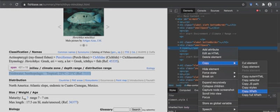
Let’s say I am interested in the Environments where Herichthys minckleyi is typically found. I run through these steps and end up with this XPATH:

//*[@id="ss-main"]/div[2]/span

I use this code to select the information I need and then repeat the process for the rest of the metadata. At the end I have a collection of XPATHS and Selectors that I can add to my function. I found that XPATHS worked best for scientific name, common name, environment, human uses, and size / weight / age metadata while Selector worked better for IUCN Red List status and threats to humans. In addition, the human uses metadata was a little tricky because on some pages it was one XPATH while on other pages it was a different XPATH. So, I had to code the threats to humans twice. Once I have the data I simply combine those columns downstream. In a nutshell, here is what this function does. Keep in mind, all of this happens behind the scenes.

Start an instance of PhantomJS & create a new browser session.
Reads a URL from the list & navigates to the site.
Goes through each of the tags, retrieves and stores the data in a data frame called article.
Moves on to the next URL and repeats.

For this function I use the command html_text, which tells rvest that I am after text.

scrape_fish_base <- function(url) {

  pjs_session$go(url)
  rendered_source <- pjs_session$getSource()
  html_document <- read_html(rendered_source)

  sci_xpath <- '//*[@id="ss-sciname"]/h1'
  sci_text <- html_document %>%
    html_node(xpath = sci_xpath) %>%
    html_text(trim = T)

  comm_xpath <- '//*[@id="ss-sciname"]/span'
  comm_text <- html_document %>%
    html_node(xpath = comm_xpath) %>%
    html_text(trim = T)

  env_xpath <- '//*[@id="ss-main"]/div[2]/span'
  evn_text <- html_document %>%
    html_node(xpath = env_xpath) %>%
    html_text(trim = T)

  threat_path <- '#ss-main > div.rlalign.sonehalf > div > span'
  threat_text <- html_document %>%
    html_node(threat_path) %>%
    html_text(trim = T)

  uses_xpath1 <- '//*[@id="ss-main"]/div[13]'
  uses_text1 <- html_document %>%
    html_node(xpath = uses_xpath1) %>%
    html_text(trim = T)

  uses_xpath2 <- '//*[@id="ss-main"]/div[12]'
  uses_text2 <- html_document %>%
    html_node(xpath = uses_xpath2) %>%
    html_text(trim = T)

  iucn_xpath <- '#ss-main > div.sleft.sonehalf > div > span'
  iucn_text <- html_document %>%
    html_node(iucn_xpath) %>%
    html_text(trim = T)

  phys_xpath <- '//*[@id="ss-main"]/div[4]/span'
  phys_text <- html_document %>%
    html_node(xpath = phys_xpath) %>%
    html_text(trim = T)

  article <- data.frame(
    url = url,
    sci_name = sci_text,
    common_name = comm_text,
    habitat = evn_text,
    threat_to_humans = threat_text,
    human_uses1 = uses_text1,
    human_uses2 = uses_text2,
    IUCN_red_list_status = iucn_text,
    physical_characters = phys_text
  )

  return(article)
}

And here is where I actually call the function.

all_fish_data <- data.frame()
for (i in 1:length(all_links)) {
  cat("Downloading", i, "of", length(all_links), "URL:", all_links[i], "\n")
  article <- scrape_fish_base(all_links[i])
  all_fish_data <- rbind(all_fish_data, article)
}

Downloading 1 of 1992 URL: https://www.fishbase.se/summary/Leucoraja-erinacea.html
Downloading 2 of 1992 URL: https://www.fishbase.se/summary/Callorhinchus-milii.html
Downloading 3 of 1992 URL: https://www.fishbase.se/summary/Latimeria-chalumnae.html
Downloading 4 of 1992 URL: https://www.fishbase.se/summary/Neoceratodus-forsteri.html
Downloading 5 of 1992 URL: https://www.fishbase.se/summary/Protopterus-aethiopicus.html

saveRDS(all_fish_data, "rdata/1_scrape_fish_base.rds")

Now I have a data frame called all_fish_data where each row is a fish species and each column is one of the metadata categories. This took a little over an hour to run through all 1992 species, but I have the slowest internet connection in the world. I expect the process would be much faster with a better connection.

Next, it is time to clean up the data. I there is a better way to code the scrape (e.g., more specific XPATHs) so less cleanup is required. Anyway, I will go through the cleanup steps for each piece of metadata.

I start with the Human Uses data. First I will make a copy of the raw data frame just in case. Here is an example of what these data look like. Remember, I had to use two different XPATHs for this metadata because of the structure of the web pages. This gets a little messy because the code picks up none-target metadata. Ok, in this example, we see that the Human uses for #4 and 5 were picked up by the first XPATH, #1, 2, and 6 by the second XPATH, while #3 returned no results.

	human_uses1	human_uses2
1	FAO(Publication : search) FishSource Sea Around Us	Fisheries: commercial
2	FAO(fisheries: production; publication : search)	Gamefish: yes; aquarium: public aquariums
3	FAO(Publication : search) FishSource	Threat to humans Harmless
4	Fisheries: subsistence fisheries	Threat to humans Harmless
5	Fisheries: minor commercial	Threat to humans Harmless
6	FAO(Publication : search) FishSource	Fisheries: subsistence fisheries

So what I needed to do was replace the non-target results with NA and then merge the two columns.

tmp_fish_data <- all_fish_data

tmp_fish_data$human_uses2  <- gsub(x = tmp_fish_data$human_uses2,
                                   pattern = "Threat to humans.*",
                                   replacement = NA)  
tmp_fish_data$human_uses1  <- gsub(x = tmp_fish_data$human_uses1,
                                   pattern = "FAO.*",
                                   replacement = NA)  
tmp_fish_data <- tmp_fish_data %>% tidyr::unite(human_uses,
                                                c(human_uses1, human_uses2),
                                                remove = TRUE, na.rm = TRUE)
tmp_fish_data$human_uses[tmp_fish_data$human_uses==""] <- NA

Next, I deal with the IUCN Red List status data. This data has some information I am not interested in (e.g., Date assessed). Here is what some of the raw data looks like.

Least Concern (LC) ; Date assessed: 27 October 2011
Vulnerable (VU) (A1c, B1+2ac); Date assessed: 01 August 1996  
Vulnerable (VU) (A1a, B1+2ac); Date assessed: 01 August 1996  
Data deficient (DD) ; Date assessed: 25 October 2011  
Vulnerable (VU) (B1+2abc, D2); Date assessed: 01 August 1996

What I want to do is remove the unwanted data and then make two columns, one for the status and another for the status abbreviation.

tmp_fish_data$IUCN_red_list_status <- stringr::str_replace(tmp_fish_data$IUCN_red_list_status,
                                                           "; Date assessed.*", "")
tmp_fish_data <- tmp_fish_data %>% tidyr::separate(IUCN_red_list_status,
                                                   into = c("IUCN", "IUCN_abr"),
                                                   sep = "[(]",  remove = TRUE)
tmp_fish_data$IUCN_abr <- stringr::str_replace(tmp_fish_data$IUCN_abr, "[)].*", "")

Moving on. Some of the Threats to Humans data has references appended (e.g., (Ref. 4537)). I am not interested in using these references for my visualization.

## threat_to_humans
tmp_fish_data <- tmp_fish_data %>% tidyr::separate(threat_to_humans,
                                                   into = c("threat_to_humans"),
                                                   sep = "[(]",  remove = TRUE)

At this point I am sad to say that I had to do the rest of the cleanup by hand, despite my best efforts to code the cleanup. The data is still pretty complicated for me to devise a suitable automated method.

write.table(tmp_fish_data, "tables/tmp_fish_data_fixed_to_manual.txt", sep = "\t", quote = FALSE)
saveRDS(tmp_fish_data, "rdata/2_scrape_fish_base_fixed_to_manual.rds")

Scrape IDs & Stock Codes

Ok, I mentioned earlier that the Distribution metadata from the main page was too difficult to parse so I decided to scrape FAO areas subpage. These pages contain a simple table that looks like this.

FAO Area	Status	Note
Indian Ocean, Western	native	30° E - 80° E; 45° S - 30° N
Indian Ocean, Eastern	native	77°E - 150°E; 55°S - 24°N
Pacific, Northwest	native

Now, the issue is that the URL for the FAO areas subpage was a bit harder to code because the links have species specific ID codes and StockCodes. Turns out that I actually needed to first scrape the main page to get the FAO areas URL then use that URL to scrape the tables.

Basically, I want to scrape the URL that is sitting under the highlighted link. As before, I first turn my list of species to FishBase URLs.

rm(list = ls())
base_url <- "https://www.fishbase.se/summary/"
fish <- scan('fish_list.txt', what = "character", sep = "\n")
rm(list = ls(pattern = "sample_data"))
sample_data <- data.frame()
for (name in fish) {
     tmp_link <- paste(base_url, name, ".html", sep = "")
     tmp_entry <- cbind(name, tmp_link)
     sample_data <- rbind(sample_data, tmp_entry)
     rm(list = ls(pattern = "tmp_"))

}
sample_data <- sample_data %>% dplyr::rename("link" = "tmp_link")

all_links <- sample_data$link
all_names <- sample_data$name

pjs_instance <- run_phantomjs()
pjs_session <- Session$new(port = pjs_instance$port)

Then I create a new function called scrape_fish_code_urls which uses the XPATH //*[@id="ss-main"]/h1[3]/span/span[2]/a to grab that subpage link. Here I use html_attr in my code to indicate that the scrape is specifically looking for a URL and not plain text.

scrape_fish_code_urls <- function(url) {

  pjs_session$go(url)
  rendered_source <- pjs_session$getSource()
  html_document <- read_html(rendered_source)

  codes_xpath <- '//*[@id="ss-main"]/h1[3]/span/span[2]/a'
  codes_text <- html_document %>%
    html_node(xpath = codes_xpath) %>%
    html_attr(name = "href", default = "https://www.fishbase.se/Country/FaoAreaList.php?ID=6320&GenusName=Herichthys&SpeciesName=minckleyi&fc=349&StockCode=6633&Scientific=Herichthys+minckleyi")

  fish_codes <- data.frame(
    url = url,
    codes = codes_text
  )

  return(fish_codes)
}

You should notice that for html_attr I used the default option and set it to a specific URL. This is an actual FAO areas page but for a species not in the list. The reason I do this is to avoid downstream errors with species that do not have a FishBase page, an FAO areas page, and/or an empty table. That way, if the code encounters a page that doesn’t exist, it will use this one instead. Poor man’s workaround to what I can only assume is a simple fix using an ifelse statement.

Again, I run the function. This time, instead of a bunch of metadata I should end up with just a new list of URLs.

all_fish_codes <- data.frame()
for (i in 1:length(all_links)) {
  cat("Downloading", i, "of", length(all_links), "URL:", all_links[i], "\n")
  fish_codes <- scrape_fish_code_urls(all_links[i])
  all_fish_codes <- rbind(all_fish_codes, fish_codes)
}

Downloading 1 of 1992 URL: https://www.fishbase.se/summary/Leucoraja-erinacea.html
Downloading 2 of 1992 URL: https://www.fishbase.se/summary/Callorhinchus-milii.html
Downloading 3 of 1992 URL: https://www.fishbase.se/summary/Latimeria-chalumnae.html
Downloading 4 of 1992 URL: https://www.fishbase.se/summary/Neoceratodus-forsteri.html
Downloading 5 of 1992 URL: https://www.fishbase.se/summary/Protopterus-aethiopicus.html

saveRDS(all_fish_codes, "rdata/3_scrape_fish_code_urls.rds")

A little clean-up is required before proceeding. I expected a full URL to the FAO pages, but instead I just got extensions. No big deal, I will just add the base URL name and make a few other changes for downstream analysis.

all_fish_codes$codes <- stringr::str_replace(all_fish_codes$codes,
                        "\\.\\./Country/FaoAreaList.php",
                        "https://www.fishbase.se/Country/FaoAreaList.php")

all_fish_codes$url <- stringr::str_replace(all_fish_codes$url, "https://www.fishbase.se/summary/", "")
all_fish_codes$url <- stringr::str_replace(all_fish_codes$url, ".html", "")
all_fish_codes <- all_fish_codes %>% dplyr::rename("name" = "url")
all_fish_codes <- all_fish_codes %>% dplyr::rename("link" = "codes")
saveRDS(all_fish_codes, "rdata/4_scrape_fish_code_urls_fixed.rds")

gdata::keep(all_fish_codes, sure = TRUE)

Scrape Distribution Tables

So now I have a new list of URLs for each species that I can use to download the FAO table data. The tables look like this.

all_links <- all_fish_codes$link
all_names <- all_fish_codes$name

pjs_instance <- run_phantomjs()
pjs_session <- Session$new(port = pjs_instance$port)

Pretty much the same function as above except this time I use the command html_table to tell rvest that I am after a table. One tricky thing is that if the table is empty the script will fail. The only way around this I could find was setting header = FALSE which treats table headers as actual data. Not a huge deal since one line of code can remove these later on.

If header = TRUE and the table is empty, the job will fail. By setting header = FALSE the function treats table headers as data. This means that the final data frame will have headers that must be removed.

scrape_fish_dist_tabs <- function(url) {

  pjs_session$go(url)
  rendered_source <- pjs_session$getSource()
  html_document <- read_html(rendered_source)
  dist_xpath <- '//*[@id="dataTable"]'
  dist_text <- html_document %>%
    html_node(xpath = dist_xpath) %>%
    html_table(header = FALSE, fill = TRUE, trim = TRUE)
  fish_dist <- data.frame(
    url = url,
    dist = dist_text
  )

  return(fish_dist)
}

all_fish_dist <- data.frame()
for (i in 1:length(all_links)) {
  cat("Downloading", i, "of", length(all_links), "URL:", all_links[i], "\n")
  fish_dist <- scrape_fish_dist_tabs(all_links[i])
  # Append current article data.frame to the data.frame of all articles
  all_fish_dist <- rbind(all_fish_dist, fish_dist)
}
saveRDS(all_fish_dist, "rdata/5_scrape_fish_dist_tabs.rds")

Downloading 1 of 1992 URL: https://www.fishbase.se/Country/FaoAreaList.php?ID=2557&GenusName=Leucoraja&SpeciesName=erinacea&fc=19&StockCode=2753&Scientific=Leucoraja+erinacea
Downloading 2 of 1992 URL: https://www.fishbase.se/Country/FaoAreaList.php?ID=4722&GenusName=Callorhinchus&SpeciesName=milii&fc=24&StockCode=4944&Scientific=Callorhinchus+milii
Downloading 3 of 1992 URL: https://www.fishbase.se/Country/FaoAreaList.php?ID=2063&GenusName=Latimeria&SpeciesName=chalumnae&fc=30&StockCode=2258&Scientific=Latimeria+chalumnae
Downloading 4 of 1992 URL: https://www.fishbase.se/Country/FaoAreaList.php?ID=4512&GenusName=Neoceratodus&SpeciesName=forsteri&fc=27&StockCode=4705&Scientific=Neoceratodus+forsteri
Downloading 5 of 1992 URL: https://www.fishbase.se/Country/FaoAreaList.php?ID=8734&GenusName=Protopterus&SpeciesName=aethiopicus&fc=552&StockCode=9056&Scientific=Protopterus+aethiopicus

What we end up with is a data frame where each line is the species URL plus a single line from the table. This means that if a table has more than one entry (like the example above), a species will have multiple entries in the data frame. I want a single entry for each species, so I need to concatenate instances of table entries.

First a little cleanup. I do not need the Note data from the tables, and I also want to change the names of the columns. I can also remove any Herichthys minckleyi since this was used as dummy data. Come to think of it, I should have removed it from the URL list before running scrape_fish_dist_tabs. Oh well, live and learn.

all_fish_dist <- readRDS("rdata/scrape_fish_dist_tabs.rds")
all_fish_dist$dist.X3 <- NULL
all_fish_dist <- all_fish_dist[all_fish_dist$dist.X1 != "FAO Area", ]
all_fish_dist <- dplyr::distinct(all_fish_dist)

all_fish_dist <- all_fish_dist %>% dplyr::rename("dist.FAO.Area" = "dist.X1")
all_fish_dist <- all_fish_dist %>% dplyr::rename("dist.Status" = "dist.X2")

Now I merge all multiple entries, so I end up with a single line per species containing the FAO area and Status.

all_fish_dist_agg <- all_fish_dist %>%
                     group_by(url) %>%
                     tidyr::pivot_wider(names_from = dist.FAO.Area,
                                    values_from = c("dist.FAO.Area",
                                                    "dist.Status"))
fao_area <- all_fish_dist_agg %>%
                  ungroup() %>%
                  dplyr::select(matches("^dist.FAO.Area_.*")) %>%
                  tidyr::unite("fao_area", na.rm = TRUE,
                               remove = TRUE, sep = "; ")

fao_status <- all_fish_dist_agg %>%
                  ungroup() %>%
                  dplyr::select(matches("^dist.Status_.*")) %>%
                  tidyr::unite("fao_status", na.rm = TRUE, remove = TRUE, sep = "; ") %>%
                  tidyr::separate(fao_status, "fao_status")

all_fish_dist_final <- cbind(all_fish_dist_agg$url, fao_area, fao_status)
write.table(all_fish_dist, "tables/temp3.txt", sep = "\t", quote = FALSE)

saveRDS(all_fish_dist_final, "rdata/6_scrape_fish_dist_tabs_final.rds")

OK! Now it is time to put everything together. Here is what I have so far.

The original species list fish_list.txt.
The manually curated metadata scrape from the species pages scrape_fish_base_final.txt.
The fixed Distance metadata from the FAO pages scrape_fish_dist_tabs_final.rds.

I read these data into R so that I can do some final touchup and merge all of the metadata.

rm(list = ls())
tree_names_dashes <- read.table("fish_list.txt", row.names = NULL)
scrape_fish_base <- read.table("tables/scrape_fish_base_final.txt",
                               header = TRUE, sep = "\t",
                               row.names = NULL, stringsAsFactors = FALSE)
scrape_dist <- readRDS("rdata/6_scrape_fish_dist_tabs_final.rds")

The trick here is that anvi’o needs a first column called id that matches the names in the tree. After that, I can list the metadata columns however I want, as long as the names are unique.

I can start by renaming the column in the names file.

tree_names_dashes <- tree_names_dashes %>% dplyr::rename("id" = 1)

Next, I will fix the data scraped from the FAO pages. This code adds a new id column and renames the other columns.

scrape_dist <- scrape_dist %>% dplyr::rename("foa_url" = 1) %>%
                               dplyr::mutate(id = foa_url, .before = foa_url)

scrape_dist$id  <- gsub(x = scrape_dist$id, pattern = "https://www.fishbase.se/Country/FaoAreaList.php\\?ID=.*Scientific=", replacement = "")
scrape_dist$id  <- gsub(x = scrape_dist$id, pattern = "\\+", replacement = "-")

scrape_fish_base <- scrape_fish_base %>% dplyr::rename("fb_url" = 1) %>%
                               dplyr::mutate(id = fb_url, .before = fb_url)
scrape_fish_base$id  <- gsub(x = scrape_fish_base$id,
                        pattern = "https://www.fishbase.se/summary/|.html",
                        replacement = "")

At this point, if I try to merge all three data frames, something will look a bit fishy. You see, the tree has 1992 species in it, yet the merged data frame has 2000 lines. So, I need to see if anything is duplicated. Sure enough, when I look at the species list I see there are 4 species that are duplicates.

tree_names_dashes[duplicated(tree_names_dashes[,1:1]),]

[1] "Opsarius-koratensis"     "Distichodus-fasciolatus" "Lactarius-lactarius"     "Banjos-banjos"

Looks like I did not notice this when I made the species list from the original tree. That’s ok. I can fix it in the final table. For now, I will remove the duplicate rows and merge all of the table.

scrape_fish_base <- dplyr::distinct(scrape_fish_base)

fish_base_merge <- dplyr::left_join(tree_names_dashes,  scrape_fish_base) %>%
                   dplyr::left_join(., scrape_dist, by = "id")
saveRDS(fish_base_merge, "rdata/7_fish_base_merge_raw.rds")

Finally, I can merge all of these metadata with my modified version of Additional file 4 (Table S1. spreadsheet with full classification) from the Betancur-R paper.

additional_data <- read.table("tables/additional_file_4_modified.txt",
                               header = TRUE, sep = "\t",
                               row.names = NULL, stringsAsFactors = FALSE)
fish_base_merge <- fish_base_merge %>% dplyr::rename("FishBase_ID" = "id")

fish_metadata <- dplyr::left_join(additional_data, fish_base_merge, by = "FishBase_ID")

fish_metadata[duplicated(fish_metadata[,1:1]),]
fish_metadata <- dplyr::distinct(fish_metadata)
fish_metadata[duplicated(fish_metadata[,1:1]),]
fish_metadata[fish_metadata==""] <- NA
saveRDS(fish_metadata, "rdata/8_fish_metadata.rds")

fish_metadata <- readRDS("rdata/8_fish_metadata.rds")
colnames(fish_metadata)
fish_metadata <- fish_metadata %>% dplyr::rename("Group" = "Betancur_R_ID")
write.table(fish_metadata, "fish_metadata_complete.txt", sep = "\t", quote = FALSE, row.names = FALSE)

fish_metadata <- fish_metadata[, -c(3:27)]
fish_metadata[, 4] <- list(NULL)
fish_metadata[, 2:5] <- list(NULL)

fish_metadata$max_reported_age  <- gsub(x = fish_metadata$max_reported_age,
                                   pattern = " years",
                                   replacement = "")  

write.table(fish_metadata, "fish_metadata.txt", sep = "\t", quote = FALSE, row.names = FALSE)

Extra Code

One last thing I wanted to (try to) do was scrape distribution data from the main species pages. Earlier I said this didn’t work but then I noticed that some species had designations like worldwide or cosmopolitan distributions. I thought it would be neat to capture these data. This ultimately didn’t work well but here is the code just in case.

#rm(list = ls())
base_url <- "https://www.fishbase.se/summary/"
fish <- scan('fish_list.txt', what = "character", sep = "\n")
rm(list = ls(pattern = "sample_data"))
sample_data <- data.frame()
for (name in fish) {
     tmp_link <- paste(base_url, name, ".html", sep = "")
     tmp_entry <- cbind(name, tmp_link)
     sample_data <- rbind(sample_data, tmp_entry)
     rm(list = ls(pattern = "tmp_"))

}
sample_data <- sample_data %>% dplyr::rename("link" = "tmp_link")

all_links <- sample_data$link
all_names <- sample_data$name

pjs_instance <- run_phantomjs()
pjs_session <- Session$new(port = pjs_instance$port)

scrape_dist <- function(url) {

  pjs_session$go(url)
  rendered_source <- pjs_session$getSource()
  html_document <- read_html(rendered_source)

  dist_xpath <- '//*[@id="ss-main"]/div[3]/span'
  dist_text <- html_document %>%
    html_node(xpath = dist_xpath) %>%
    html_text(trim = T)

  article <- data.frame(
    url = url,
    distribution = dist_text
  )

  return(article)
}

dist_data <- data.frame()
for (i in 1:length(all_links)) {
  cat("Downloading", i, "of", length(all_links), "URL:", all_links[i], "\n")
  article <- scrape_dist(all_links[i])
  # Append current article data.frame to the data.frame of all articles
  dist_data <- rbind(dist_data, article)
}

saveRDS(dist_data, "rdata/9_scrape_fish_base_just_dist.rds")
write.table(dist_data, "tables/scrape_fish_base_just_dist.txt", sep = "\t", quote = FALSE)

Scape Conclusion

Unfortunately I had to do quite a bit of post-processing to the scraped data because I couldn’t figure out how to do it in R. Oh well.

Adding Microbiome Data

There are two more pieces of information I want to add. The first is to identify fish that have been analyzed for microbiome content. To accomplish this, I used pysradb, a python package for retrieving metadata and downloading datasets from NCBI’s Sequence Read Archive (SRA) and/or the European Nucleotide Archive (ENA). To simplify things, I decided to search for genus only, rather than include the species name. The first thing I needed was a list of all fish genera.

tmp_fish_list <- read.delim("tables/additional_file_4_modified.txt", header = TRUE)
tmp_fish_list <- dplyr::filter(tmp_fish_list, CLADE != "OUTGROUP")
tmp_fish_list <- data.frame(tmp_fish_list$Betancur_R_ID)
tmp_fish_list <- data.frame(stringr::str_split_fixed(tmp_fish_list[[1]], "_", 3))
tmp_fish_list[,2:3] <- NULL
tmp_fish_list <- unique(tmp_fish_list)
write.table(tmp_fish_list, "fish_list_genera.txt", row.names = FALSE,
            quote = FALSE, col.names = FALSE)

Then I used a for loop to cycle through each genus in the list to fetch metadata from the SRA and ENA.

for NAME in `cat fish_list_genera.txt`

do
    pysradb search --query $NAME --db sra -v 3  \
                   --saveto $NAME-sra-hits.txt \
                   --max 20 --stats > $NAME-sra-stats.txt
    pysradb search --query $NAME --db ena -v 3  \
                   --saveto $NAME-ena-hits.txt \
                   --max 20 --stats > $NAME-ena-stats.txt
done

Now I had two text files for each genus from both the SRA and ENA, so four files total. The ENA and SRA capture slightly different information. I wanted to make sure I wasn’t missing anything, so I searched both. I began with the stats file, which provide some basic information about each search term. My plan was to use these files to identify hits that had certain keywords that would indicate some type of microbiome analysis. Here is an example of this file from the genus Acanthurus.

  Statistics for the search query:
  =================================
  Number of unique studies: 5
  Number of unique experiments: 20
  Number of unique runs: 20
  Number of unique samples: 20
  Mean base count of samples: 682131524.950
  Median base count of samples: 1000023.500
  Sample base count standard deviation: 1733608136.332
  Date range:
	  2015-01:  16
	  2016-07:  1
	  2017-02:  1
	  2017-06:  1
	  2020-10:  1

  Organisms:
	  Acanthurus bahianus:  1
	  Acanthurus mata:  1
	  Varanus acanthurus:  1
	  gut metagenome:  17

  Platform:
	  ILLUMINA:  4
	  LS454:  16

  Library strategy:
	  AMPLICON:  16
	  RNA-Seq:  3
	  Targeted-Capture:  1

  Library source:
	  GENOMIC:  1
	  METAGENOMIC:  16
	  METATRANSCRIPTOMIC:  1
	  TRANSCRIPTOMIC:  2

  Library selection:
	  Hybrid Selection:  1
	  PCR:  16
	  RANDOM:  2
	  cDNA:  1

  Library layout:
	  PAIRED:  4
	  SINGLE:  16

Some of this information—like Organisms, Library strategy, Library source—will be useful while others (e.g., Date range) will not.

Unfortunately, the structure of the file is a bit clunky and I had to write some equally clunky code to create a usable table. Step one was to reformate each file and then merge them all into a single dataframe.

no_results <- "No results found for the following search query"
pysradb_results <- NULL
pysradb_files <- list.files(path = "pysradb_results", pattern = "*.txt",
                            full.names = TRUE, recursive = FALSE)
for (i in pysradb_files) {
    tmp_fish <- read_file(i)

    if(isTRUE(grepl(no_results, tmp_fish, fixed = TRUE)))
      next
    tmp_fish <- gsub(": \n\t  ", "---", tmp_fish)
    tmp_fish <- gsub(":  ", " (", tmp_fish)
    tmp_fish <- gsub("\n\t  ", ");", tmp_fish)
    tmp_fish <- gsub("\n\n  ", ")\n  ", tmp_fish)
    tmp_fish <- gsub(": ", "---", tmp_fish)
    tmp_fish <- data.frame(strsplit(tmp_fish, split = "\n  "))
    tmp_fish <- data.frame(tmp_fish[-c(1:3), ])
    tmp_fish <- data.frame(tmp_fish) %>%
                  dplyr::rename("id" = 1)
    tmp_fish$id <- gsub("\n+", ")", tmp_fish$id)

    tmp_fish <- data.frame(stringr::str_split_fixed(tmp_fish$id, "---", 2)) %>%
          dplyr::rename("metric" = 1) %>%
          dplyr::rename("results" = 2)
    tmp_str <- i
    tmp_str <- str_remove(tmp_str, "pysradb_results/")
    tmp_str <- stringr::str_split_fixed(tmp_str, pattern = "-", n = 3)

    tmp_fish$genus <- tmp_str[1]
    tmp_fish$db <- tmp_str[2]
    tmp_fish <- tmp_fish[,c(3,4,1,2)]
    pysradb_results <- rbind(pysradb_results, data.frame(tmp_fish))
    rm(list = ls(pattern = "tmp_"))
}
dplyr::filter(pysradb_results, metric == "Library source")

A little more reformating.

pysradb_results_wide <- tidyr::pivot_wider(pysradb_results,
                                           names_from = metric,
                                           values_from = results)
pysradb_results_wide <- pysradb_results_wide %>%
                        dplyr::rename(unique_studies = 3,
                                      unique_experiments = 4,
                                      unique_runs = 5,
                                      unique_samples = 6,
                                      mean_base_count = 7,
                                      median_base_count = 8,
                                      sd_base_count = 9,
                                      date_range = 10,
                                      organisms = 11,
                                      platform = 12,
                                      library_strategy = 13,
                                      library_source = 14,
                                      library_selection = 15,
                                      library_layout = 16)
pysradb_results_wide <- pysradb_results_wide[,c(1:2,11,14,13,3:9,12,15,16,10)]
write.table(pysradb_results_wide, "pysradb_results_wide.txt",
                                   row.names = FALSE, quote = FALSE, sep = "\t")

And we get a single dataframe containing the summary stats from both databases for every genus. Any genus not found in either data base is absent from the table.

Here is an abbreviated version of the metadata scraped from the sequence read archives.

genus	db	organisms	library_source	library_strategy	platform	library_selection	library_layout
Abudefduf	ena	fish gut metagenome (20)	METAGENOMIC (20)	AMPLICON (20)	ILLUMINA (20)	PCR (20)	SINGLE (20)
Acanthochromis	ena	Acanthochromis polyacanthus (8);fish gut metagenome (12)	METAGENOMIC (12);TRANSCRIPTOMIC (8)	AMPLICON (12)	ILLUMINA (20)	PCR (12);cDNA (8)	PAIRED (8);SINGLE (12)
Acanthurus	ena	Acanthurus bahianus (1);gut metagenome (17)	METAGENOMIC (16);METATRANSCRIPTOMIC (1)	AMPLICON (16)	ILLUMINA (4);LS454 (16)	PCR (16);RANDOM (2);cDNA (1)	PAIRED (4);SINGLE (16)
Acanthurus	sra	Acanthurus bahianus (2);gut metagenome (11)	GENOMIC (3);METAGENOMIC (16)	AMPLICON (10);WGS (6)	ILLUMINA (20)	PCR (15);PolyA (1);RANDOM (2)	PAIRED (13);SINGLE (7)
Acheilognathus	sra	Acheilognathus tonkinensis (1);metagenome (2)	GENOMIC (1);METATRANSCRIPTOMIC (2)	AMPLICON (1)	ILLUMINA (3)	PCR (1);RANDOM (2)	PAIRED (3)
Achirus	sra	Achirus lineatus (8);metagenome (12)	METAGENOMIC (12);TRANSCRIPTOMIC (8)	AMPLICON (12)	ILLUMINA (20)	PCR (12);RT-PCR (8)	PAIRED (20)
Aethaloperca	ena	coral reef metagenome (1)	GENOMIC (1)	AMPLICON (1)	ILLUMINA (1)	PCR (1)	PAIRED (1)

We ended up with 1,659 total hits—divide that by 2 mean we retrieved information for roughly 830 genera. However, a lot of these molecular studies have nothing to do with microbes. After scanning the table, I decided to start by selecting studies that generated data from either METATRANSCRIPTOMIC or METAGENOMIC libraries. I also used several keywords like fish, gut, etc.

pysradb_trim <- pysradb_results_wide[(
                      grepl("METATRANSCRIPTOMIC", pysradb_results_wide$library_source) |
                      grepl("METAGENOMIC", pysradb_results_wide$library_source) |
                      grepl("fish", pysradb_results_wide$organisms) |
                      grepl("metagenome", pysradb_results_wide$organisms) |
                      grepl("gut", pysradb_results_wide$organisms)), ]

This gave me 326 hits. I then removed any exact duplicates between ena and sra data.

tmp_check <- c("genus","organisms","library_source","library_strategy",
               "unique_studies","unique_experiments","unique_runs",
               "unique_samples","platform","library_selection",
               "library_layout")
pysradb_trim <- pysradb_trim[!duplicated(pysradb_trim[,tmp_check]),]
#tmp_trim <- tmp_trim[!duplicated(tmp_trim[,c('organisms','genus')]),]

Which reduced the total number to 309 hits. Now I wanted to check whether the genus name is actually in the organisms column. When you search the archives using pysradb, I am pretty sure the algorithum is using a fuzzy seach, meaning when you search for something like Acanthocobitis you will also get hits for Paracanthocobitis—both fish, but something like Albula will also hit Galbula, which is a jacamar. I am uncertain how to perform exact searches with pysradb but I am sure it is possible. Anyway, the code below will look for the genus name in the organism column, then add a new column with the results (TRUE/FALSE) of the query.

check_org_name <- NULL
for (i in 1:nrow(pysradb_trim)) {
  tmp_check <- grepl(pysradb_trim$genus[i], pysradb_trim$organisms[i])
  check_org_name <- rbind(check_org_name, data.frame(tmp_check))
  rm(list = ls(pattern = "tmp_"))
}
tmp_match <- cbind(check_org_name, pysradb_trim)

193 hits returned a value of TRUE and 116 were FALSE. Remember, I am screening two databases—the ENA and SRA—so in the table, I have search terms that were either found in the organism description for both databases, neither database, or only one database. I need to separate all of this out. I start with the genera that were either found in both or not found in both.

tmp_match_dup <- tmp_match[tmp_match$genus %in%
                            tmp_match$genus[
                              duplicated(tmp_match[, c("genus",
                                                       "tmp_check")])],]
tmp_match_dup_t <- tmp_match_dup %>% dplyr::filter(tmp_check == "TRUE")
good_list_1 <- tmp_match_dup_t[duplicated(tmp_match_dup_t[,c('genus')]),]

tmp_match_dup_f <- tmp_match_dup %>% dplyr::filter(tmp_check == "FALSE")

This screening gives me 30 unique hits that were TRUE and 24 total hits that were FALSE. Now for the rest of the data.

tmp_match_no_dup <- tmp_match[!tmp_match$genus %in%
                            tmp_match$genus[
                              duplicated(tmp_match[, c("genus",
                                                       "tmp_check")])],]
good_list_2 <- tmp_match_no_dup %>% dplyr::filter(tmp_check == "TRUE")
tmp_match_no_dup_f <- tmp_match_no_dup %>% dplyr::filter(tmp_check == "FALSE")

OK. 133 unique hits that were TRUE and 92 unique hits that were FALSE. At this point, I have 163 hits that have one of the filtering terms described above AND have the search term in the organism description. Now I need to deal with all of the hits that do not have the search term in the organism description. For this I again go back and select any organism descriptions that have either fish or coral, and I get 43 more hits.

tmp_filt <- tmp_match_dup_f[(
                      grepl("fish", tmp_match_dup_f$organisms) |
                      grepl("coral", tmp_match_dup_f$organisms)), ]
good_list_3 <- tmp_filt[duplicated(tmp_filt[,c('genus')]),]
tmp_filt <- tmp_match_dup_f[!(
                      grepl("fish", tmp_match_dup_f$organisms) |
                      grepl("coral", tmp_match_dup_f$organisms)), ]
good_list_4 <- tmp_match_no_dup_f[(
                      grepl("fish", tmp_match_no_dup_f$organisms) |
                      grepl("coral", tmp_match_no_dup_f$organisms)), ]

good_list_5_unscreened <- tmp_match_no_dup_f[!(
                      grepl("fish", tmp_match_no_dup_f$organisms) |
                      grepl("coral", tmp_match_no_dup_f$organisms)), ]

write.table(good_list_5_unscreened, "good_list_5_unscreened.txt",
                                   row.names = FALSE, quote = FALSE, sep = "\t")

search_res <- NULL
search_files <- list.files(path = "PICK_ENA", pattern = "*.txt",
                            full.names = TRUE, recursive = FALSE)
for (i in search_files) {
  tmp_term <- stringr::str_split(i, "-", 2)
  tmp_term <- stringr::str_split(tmp_term[[1]][1], "/", 2)
  tmp_term <- tmp_term[[1]][2]
  tmp_grep <- grepl(tmp_term, readLines(i))
  tmp_hit <- "TRUE" %in% tmp_grep
  tmp_res <- data.frame(cbind(tmp_term, tmp_hit))
  search_res <- rbind(search_res, data.frame(tmp_res))
  rm(list = ls(pattern = "tmp_"))
}  
ena_true <- dplyr::filter(search_res, tmp_hit == "TRUE")

ena_true$tmp_term %in% sra_true$tmp_term
dplyr::full_join(sra_true, ena_true, by = "tmp_term")

good_list_5_list <- list.files(path = "PICK", pattern = "*.txt",
                            full.names = FALSE, recursive = FALSE)
good_list_5_list <- data.frame(gsub(x = good_list_5_list,
                                   pattern = "-[a-z]{3}-hits.txt",
                                   replacement = "")) %>%
                   dplyr::rename("genus" = 1)

good_list_5 <- dplyr::left_join(good_list_5_list, good_list_5_unscreened)

good_df <- rbind(good_list_1, good_list_2, good_list_3, good_list_4, good_list_5)
good_df <- good_df %>% arrange(genus)
good_df <- good_df %>% tibble::remove_rownames()
good_df$tmp_check <- NULL
good_list <- data.frame(good_df$genus)

After some manual inspection and other data wrangling, I end up with a final list of 240 unique genera that I am pretty confident has some associated microbiome data.

It looks like this:

genus	microbiome
Abudefduf	yes
Acanthochromis	yes
Acanthurus	yes
Acheilognathus	yes
Albula	yes

Fish of Panama

The last piece of the puzzle I wanted to add was which fish have been recorded from Panama. For this, I scraped the Fish of Panama checklist from STRI. My method was similar to my scrape of FishBase described above.

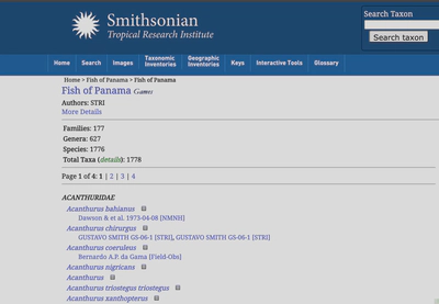
What I am after here is simply a list of species identified from Panama. The check list spans four separate pages, so the code will go through each page and grad the text associated with a specifc XPATH.

page_numbers <- 1:4
base_url <- "https://stricollections.org/portal/checklists/checklist.php?pagenumber="
paging_urls <- paste0(base_url, page_numbers, "&clid=4&dynclid=0&showvouchers=1&pid=4&searchsynonyms=1")

scrape_stri_fish <- function(url) {

  pjs_session$go(url)
  rendered_source <- pjs_session$getSource()
  html_document <- read_html(rendered_source)

  body_xpath <- '//*[contains(concat( " ", @class, " " ), concat( " ", "taxon-span", " " ))]'
  body_text <- html_document %>%
    html_nodes(xpath = body_xpath) %>%
    html_text(trim = T)

  article <- data.frame(
    id = body_text
  )

  return(article)

}

all_articles <- data.frame()
for (i in 1:length(paging_urls)) {
  cat("Downloading", i, "of", length(paging_urls), "URL:", paging_urls[i], "\n")
  article <- scrape_stri_fish(paging_urls[i])
  # Append current article data.frame to the data.frame of all articles
  all_articles <- rbind(all_articles, article)
}
panama_fish <- all_articles
panama_fish <- data.frame(stringr::str_split_fixed(panama_fish$id, " ", 3))
panama_fish[,3] <- NULL
panama_fish$id <- paste(panama_fish[[1]], panama_fish[[2]], sep = "_")
panama_fish[,1:2] <- NULL
panama_fish$Panama <- "yes"

genus	Panama
Acanthurus_bahianus	yes
Acanthurus_chirurgus	yes
Acanthurus_coeruleus	yes
Acanthurus_nigricans	yes
Acanthurus_triostegus	yes

Merge these data with the microbiome data and I am done.

panama_fish
panama_fish <- panama_fish %>% arrange(id)
good_list$microbiome <- "yes"
good_list <- good_list %>% dplyr::rename("genus" = 1)
merge_list <- read.table("merge_list.txt",
                               header = TRUE, sep = "\t",
                               row.names = NULL)
panama_fish

tmp_merge <- dplyr::left_join(merge_list, panama_fish)

tmp_merge[duplicated(tmp_merge$items),]
tmp_merge <- dplyr::distinct(tmp_merge)
tmp_merge2 <- dplyr::left_join(tmp_merge, good_list)
tmp_merge2[duplicated(tmp_merge2$items),]

profile_db_add <- dplyr::distinct(tmp_merge2)

Now I have a tree and gobs of associated metadata. Time to visualize so let’s talk about anvi’o.

Visualizations in anvi’o

First of all, if you have never used anvi’o, you need to install it. Anvi’o is really easy to install using conda in the Miniconda environment. See the installation instructions here. Once installed, run the following command:

anvi-self-test --suite mini

If you do not get any error you’re good to go.

In order to use anvi’o for the visualization, I need three files:

A tree, in this case the Betancur-R tree I modified.
A metadata file where the row names match the names in the Betancur-R tree exactly.
An anvi’o profile database.

Since we do not have a profile database, we can let anvi’o create a database for us.

anvi-interactive --profile-db profile.db \
                 --view-data metadata.txt \
                 --tree collapsed_fish_tree.tre
                 --manual

This command will open a new window in your browser where you can explore the tree and associated metadata. Done. Bye :)